Thanks to Yifeng Wu for contributing the section on rendering output.

One of Sigma’s major features is the ability to export data from workbooks to various formats such as CSV, Excel, and Google Sheets. In addition to exporting data on demand, Sigma makes it easy to build automations that run scheduled exports when a given condition is met, and deliver reports via email, Slack, or even webhooks that power our users’ business workflows.

A key component of our infrastructure that powers data exports is our backend service that consumes the results of queries from our users’ cloud data warehouses and transforms them into a variety of formats. This service is written in Rust and is designed to crunch through large amounts of data using the Apache Arrow memory format. Let’s take a look at how the result transformation service works. In particular, we’ll look at how Sigma exports pivot tables.

What is a pivot table?

Sigma offers several types of tables and visualizations to enable business users to gain insights from their data. A pivot table is a particular type of visualization that displays aggregated values from an underlying table, which have been grouped into various categories.

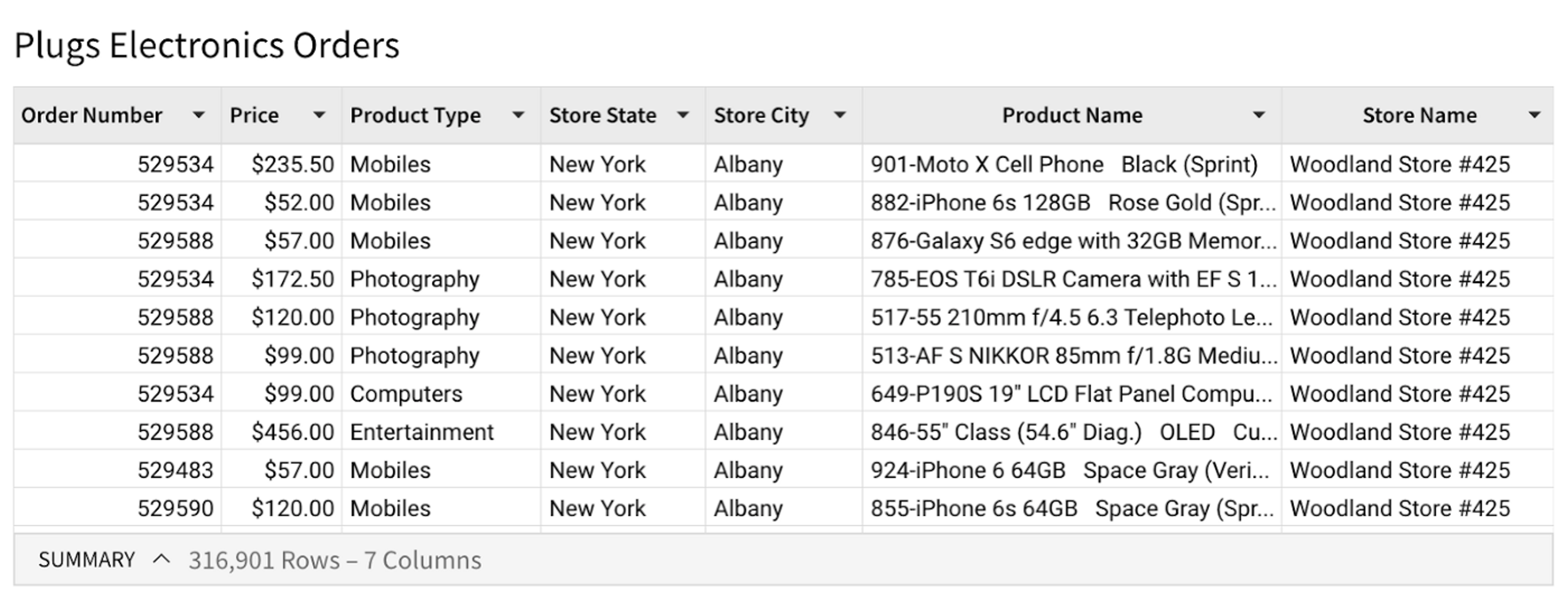
For example, suppose we start with the following table, containing order data for a chain of electronics stores.

Suppose we want to find out the total price among all orders in every city and state, across each product category. The following pivot table gives us that information.

Several parameters determine a pivot table’s layout:

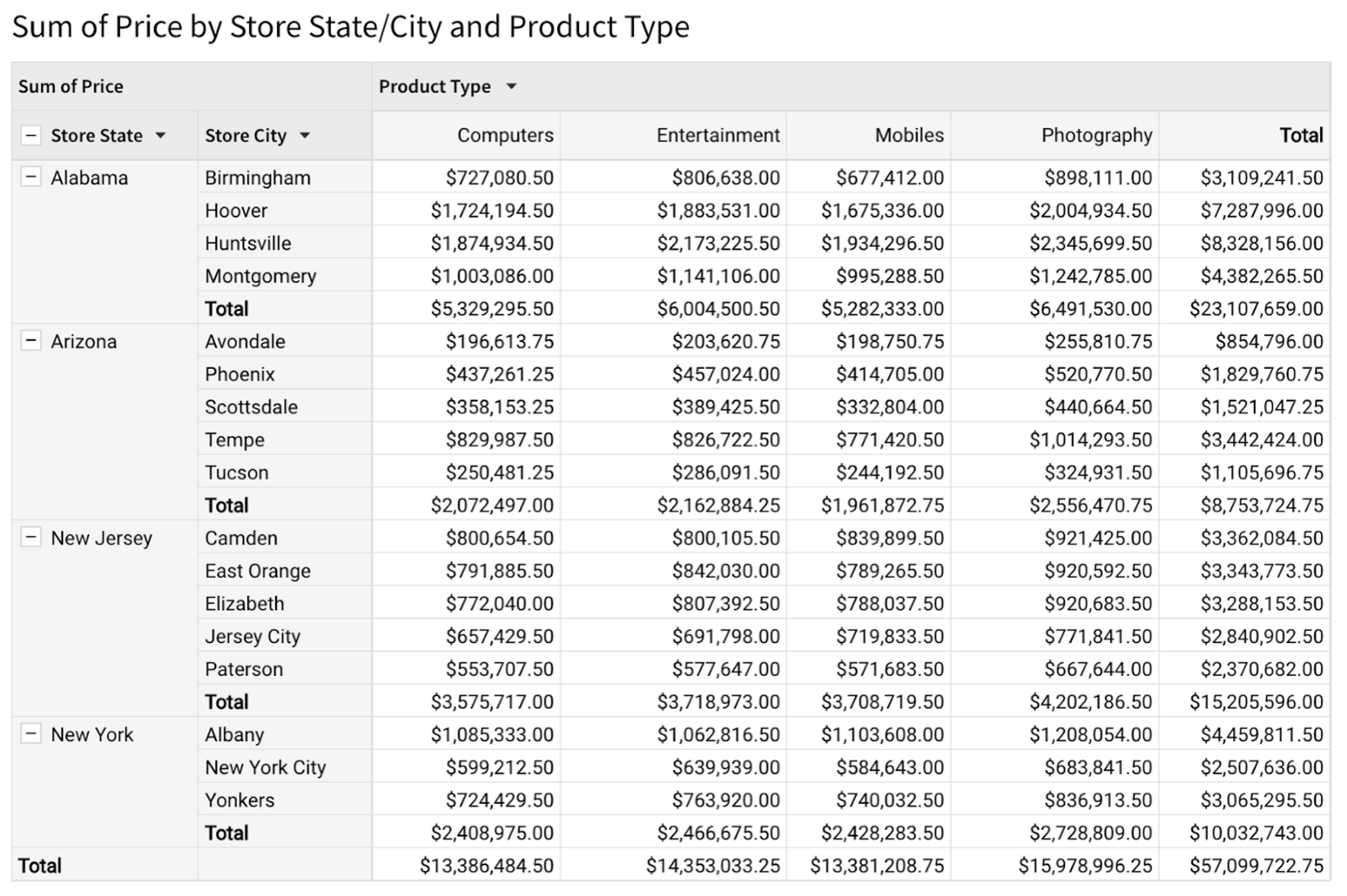
• The row dimensions are the columns from the underlying table used to group data appearing along the vertical axis of the pivot table. Here, the row dimensions are Store State and Store City.
• The column dimensions, like the row dimensions, specify the columns from the underlying table used to group data appearing along the horizontal axis of the pivot table. In this example we have one column dimension, Product Type.
• The value (or measure) is the column from the underlying table that we are aggregating. In this case, it’s the sum of prices within each grouping.

In general, a pivot table’s layout can be arbitrarily complex, with any number of row dimensions, column dimensions, and measures. Our pivot tables also support displaying subtotals, which give us aggregated values at various levels of grouping. For example, the pivot table above shows the total price for each city, state, and product type, along with a grand total.

Computing pivot table exports

There are several steps that go into building and exporting a pivot table to a format like Excel or CSV:

1. Aggregating the underlying data using SQL,
2. Computing a pivot index that represents the pivot table’s grid layout, and
3. Rendering the output in the requested format.

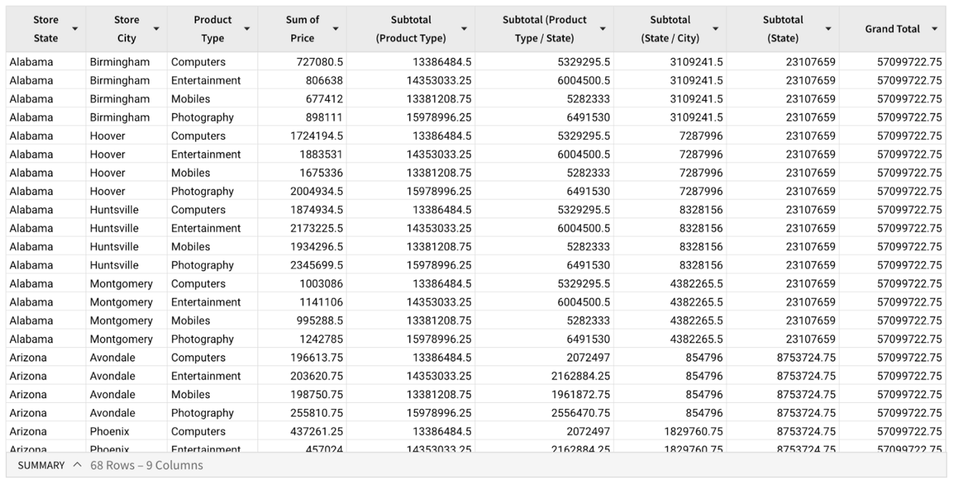
The first step is to group the data according to the specified dimensions and compute the aggregated values. The computation for this step doesn’t actually run in Sigma’s backend services. Instead, it runs as a SQL query that Sigma generates, which gets executed in the cloud data warehouse where the data is stored.

For the example above, our query compiler would generate a SQL query that produces the following output, containing the grouping dimensions (Store State, Store City, and Product Type), the aggregated pivot value column (Sum of Price), along with subtotals computed at various grouping levels.

Generating the SQL to compute the values in the pivot table is handled by our query compiler service, and is a topic that deserves its own in-depth examination. For now, we’ll focus specifically on how we transform the grouped and aggregated table that we receive from the data warehouse into a pivot table in the desired output format.

Once we have a table containing the grouped and aggregated data, the next step is to arrange the values in the shape of a pivot table, with grouping labels displayed along the vertical and horizontal axes. To do this, we build up a pivot index data structure that encodes the pivot table’s layout in a manner that’s efficient and independent of the target file type or style.

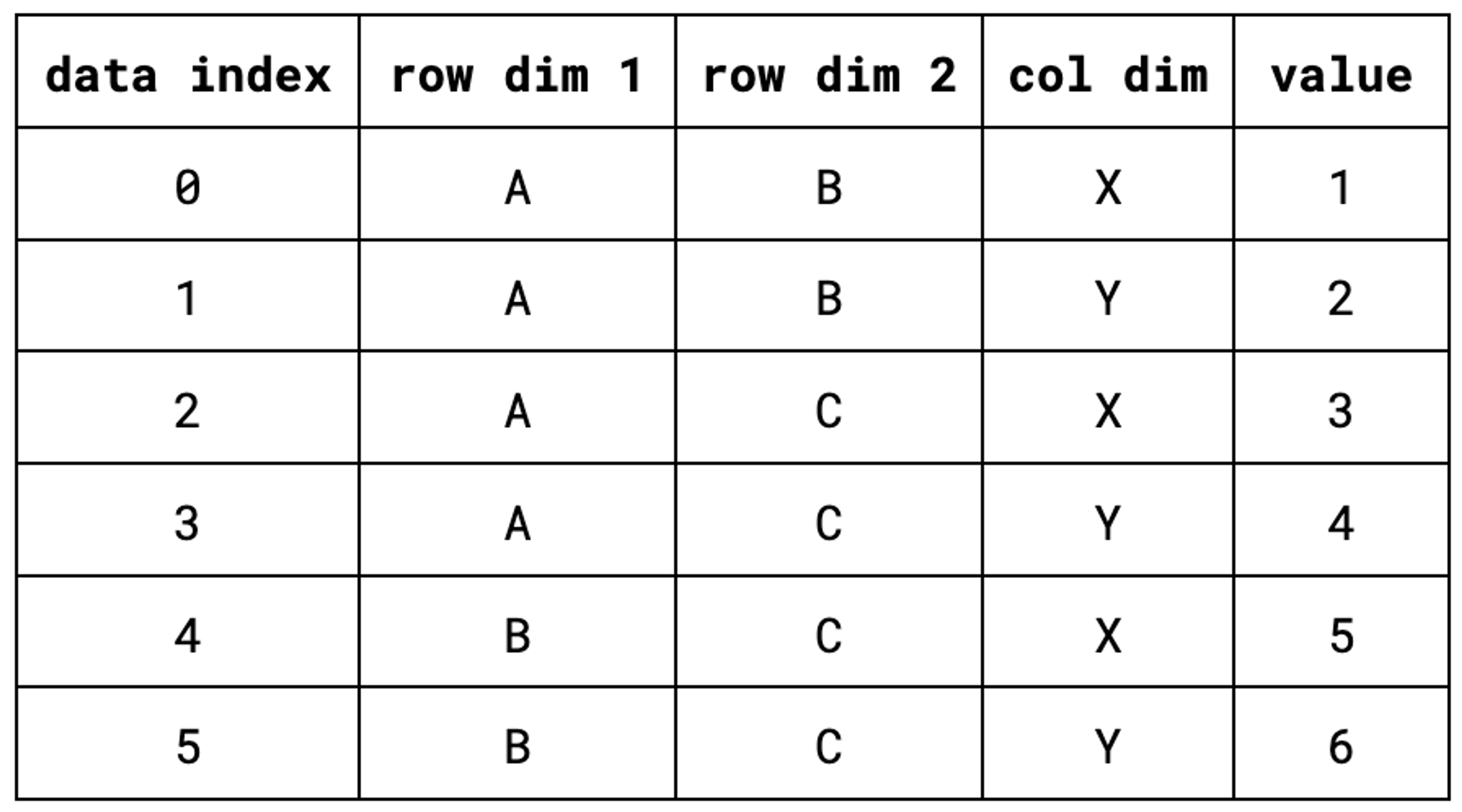
Let’s walk through a small example. Suppose we start with an aggregated table from our data warehouse containing two row dimensions, one column dimension, and one value column.

The first step is to compute a pair of sort indexes for the data: One for the row dimensions, and one for the column dimensions. A sort index is a permutation of the data indices of an array that lets us iterate over the array as though it were sorted according to the value of a particular field, without actually sorting the underlying data.

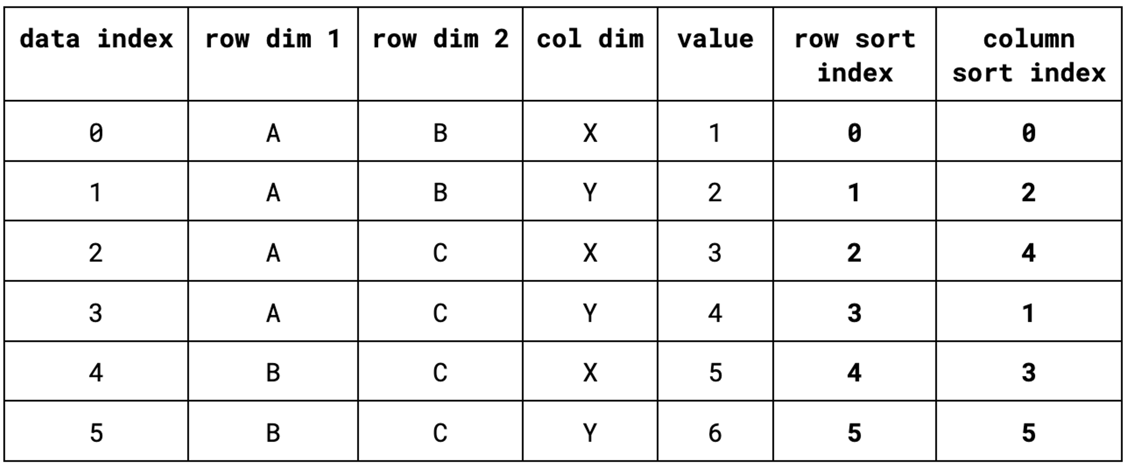
In this example, the data is already sorted according to the first row dimension, with ties being broken by the second row dimension, so the row sort index would simply be the identity permutation [0, 1, 2, 3, 4, 5]. On the other hand, the column sort index would be [0, 2, 4, 1, 3, 5], that is, the indices of all of the records containing X in the column dimension, followed by the ones that have a column dimension value of Y. Below, we have the same table as above, but with the sort indexes added as columns.

Once we have the sort indexes, we compute a pivot index. This is a data structure that efficiently summarizes the layout of a pivot table. A pivot index consists of a set of label indexes for each of the row and column dimensions, along with a values index. The values index is pretty simple: It maps pairs of horizontal and vertical offsets (coordinates in the resulting pivot table) to the rows in the underlying table where their corresponding values can be found.

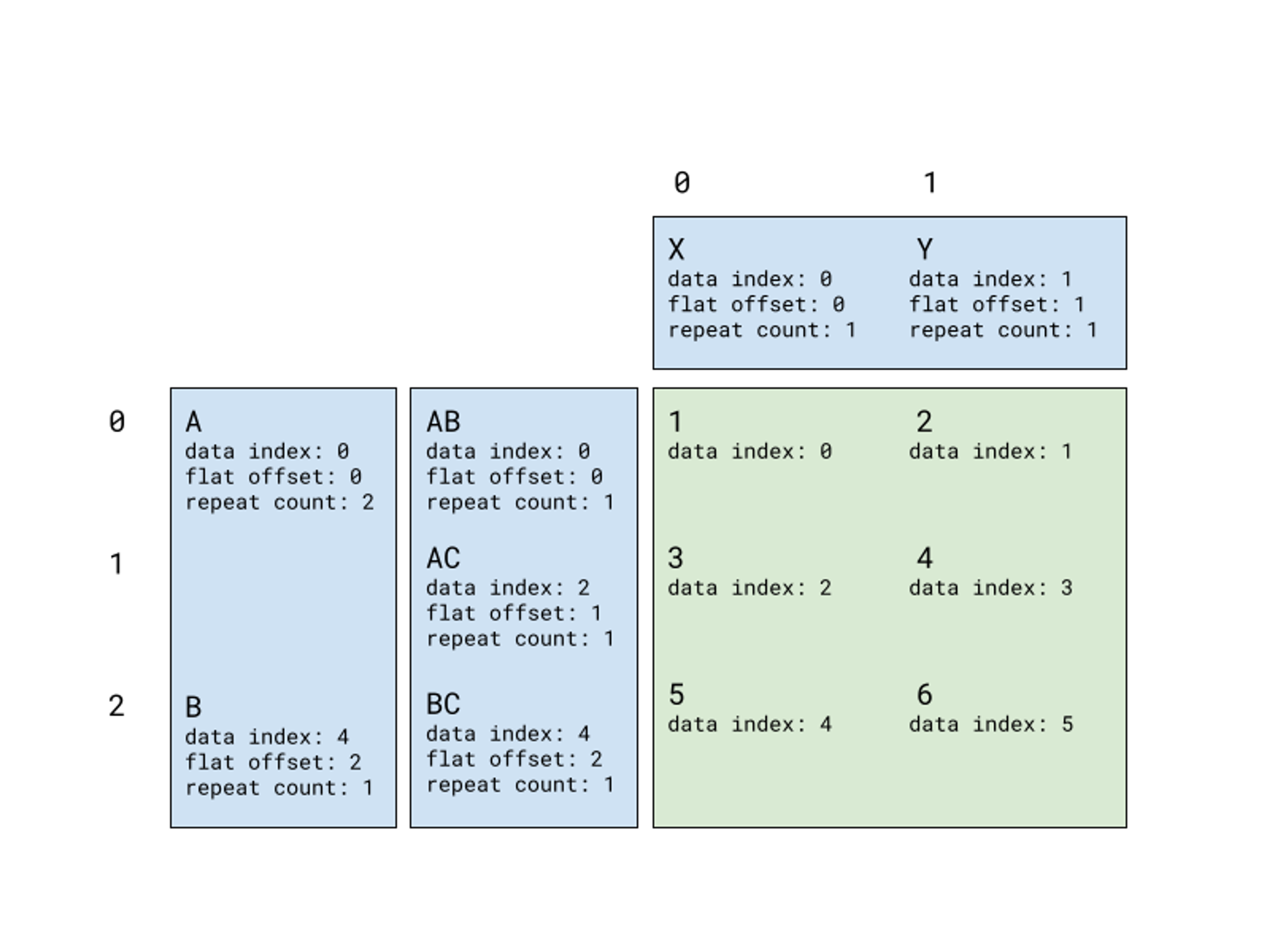
A label index represents the labels that we display for each grouping dimension. For each dimension, we store a list of label entries, where each entry stores the following information:

1. The index in the underlying data where the label’s value can be found,
2. The label’s flat offset, that is, the label’s position along either the horizontal or vertical axis,
3. A repeat count, so that we don’t have to store lots of repeated entries.

For the table above, we can visualize the pivot index using the following diagram:

In this diagram, the blue boxes represent the label indexes, while the green box represents the values index. For example, the label entry containing the value B for the first row dimension refers to a data index of 4 (the first row in which B appears in the first row dimension column), with a flat offset of 2, and a repeat count of 1, since it only has one sub-group. On the other hand, the entry for A has a repeat count of 2, since there are two sub-groups corresponding to its value.

To reduce the amount of copying we need to do, the pivot index does not store the actual values as they appear in the data, but rather works with references into the underlying table’s memory.

Our result transformation service is built using Rust’s asynchronous Tokio runtime, which enables a single replica of the service to handle thousands of concurrent requests with a small number of threads.

Although we’ve tried to make the pivot index computation as efficient as possible, computing a pivot index for a large table is still a fairly CPU-intensive process. Because we only allocate a small number of threads to handling incoming requests, we need to ensure that computing a large pivot index doesn’t block other tasks from running. To ensure that other tasks are able to make progress, we use Tokio’s spawn_blocking primitive to execute index computation tasks on a separate thread pool from the one that’s responsible for handling incoming API requests.

Rendering the output

Once we have the pivot index, we have everything we need to create a pivot table. The next step is to use the pivot index along with the aggregated table to render the output in the user’s chosen format.

To support multiple export formats, we built several pivot serializers that consume a pivot index along with the aggregated table above. They output either a CSV or Excel file, or they upload the data to Google Sheets via their API. To facilitate code reuse within our pivot serializer module, we use a variation on the Visitor design pattern to build serializers that can render the data encoded in a pivot index using a variety of output formats. This is made up of a couple of pieces.

The first is a visitor interface that specifies methods such as visit_boolean, visit_string, etc., which can be implemented to write cells of a pivot table in a given format. We have separate implementations of this visitor for CSV, Excel, and Google Sheets.

The second piece is an export_pivot() method that accepts a visitor and a pivot index. This method iterates through each cell in the pivot table. During each visit, we execute the following steps:

1. Retrieve the cell’s value using the pivot index and the aggregated table.
2. Retrieve the cell context from the pivot index. The cell context describes everything we need to know to render a particular cell, apart from its value. This includes the cell’s location in the table (i.e. whether it’s a header or a measure value), its repeat count, and a reference to the column of the aggregated table where the values come from.
3. Call the appropriate visitor method with a cell’s value, its cell context, and its location in the resulting pivot table.

During the rendering step, we also apply any formatting options that the user has specified. For example, Sigma supports a variety of number formatting options that can be applied to the cells of a pivot table. In the case of Excel, we also leverage the wide variety of formatting options that Excel provides, such as merging cells, text formatting, and alignment.

The rendering step for Google Sheets differs slightly from those of CSV and Excel, mainly because instead of producing a file that the user downloads, we write the data to Google Sheets using their API. As such, the output of the rendering step consists of a list of batch update API calls to perform tasks like creating the sheet, writing data, and merging cells, which then get executed on the user’s Google Sheets account.

Conclusion

This post just scratches the surface, but we hope that this gives you an idea of some of the exciting challenges that Sigma’s engineering team works on! If you found this interesting, we’d love for you to check out or open positions, and apply to work with us!

Thanks to James Johnson

‍